Open-Source Flood Frequency Analysis for ARR 2019: My pyextremes Fork
The flood frequency analysis space in Python has a gap. Georgy Bocharnikov’s pyextremes is a well-engineered extreme value analysis library — block maxima, peaks-over-threshold, return value plots, confidence intervals. But it doesn’t natively support the Log-Pearson Type III distribution, Multiple Grubbs-Beck Test for low-outlier censoring, or LH-moments — the three tools that Australian practitioners need to comply with ARR 2019 Book 3 and USGS Bulletin 17C at-site flood frequency analysis.
I’ve been building those additions in a fork: lmillard79/pyextremes, branch ARR2019_Book3.
The branch is functional and testable now. I’m not ready to submit a pull request to the upstream repository — ARR 2019 specifics may be outside the original library’s scope — but if you work in Australian flood hydrology and want a pure-Python FFA workflow that actually aligns with our standards, this is worth looking at. Bug reports and feedback via GitHub Issues are genuinely useful.
The Gap This Fills
Standard Python EVA tools give you GEV and Gumbel distributions, which are appropriate for coastal or European hydrology contexts. Australian at-site flood frequency analysis under ARR 2019 uses:
- LP3 (Log-Pearson Type III) — the primary at-site distribution, recommended by ARR 2019 Book 3 Chapter 2 and Bulletin 17C
- PILF censoring via Multiple Grubbs-Beck Test — excluding Potentially Influential Low Floods that distort upper tail estimation
- TCEV (Two-Component Extreme Value) — for catchments where floods arise from two distinct physical mechanisms
- LH-moments — higher-order L-moments that address the “separation effect” in Australian streamflow data
None of these were available in pyextremes. They are now.
1. Log-Pearson Type III Distribution
LP3 is Australia’s workhorse at-site distribution — fitting it via L-moments (rather than product-moments) gives more robust parameter estimates for the short records typical of Australian gauges.
import pandas as pd
from pyextremes import EVA

model = EVA(data=streamflow_series)
model.get_extremes(method="BM", block_size="1Y")

# Fit LP3 using L-moments (ARR 2019 recommended approach)
model.fit_model(
    model="Lmoments",
    distribution="logpearson3"
)
L-moment fitting is computationally stable and less sensitive to extreme outliers than MLE, which matters when fitting to a 30–50 year gauge record that may include one or two anomalously large events.
2. Multiple Grubbs-Beck Test — PILF Identification
Low outliers in a flood record are not just small floods. They represent events from a different population — low-antecedent-moisture or partial-duration threshold events — that can dominate statistical fit and produce parameters that underestimate the upper tail. The Multiple Grubbs-Beck Test (MGBT) identifies these Potentially Influential Low Floods and removes them from the fitting dataset.
from pyextremes.tuning.outliers import multiple_grubbs_beck

# Identify and remove PILFs at 10% significance level
censored_extremes = multiple_grubbs_beck(model.extremes, alpha=0.10)
print(f"Removed {len(model.extremes) - len(censored_extremes)} PILFs from the fit dataset")

model.extremes = censored_extremes
This is directly analogous to the sensitivity analysis approach used in the 2024 Kedron Brook Flood Study — where excluding the 2022 events tests whether the record is being dominated by a small number of large values. MGBT is the automated version of that test, applied to the lower tail.
3. TCEV — Two-Component Extreme Value Distribution
The TCEV distribution is appropriate when a catchment’s flood record is drawn from two distinct physical mechanisms — for example, in North Queensland where tropical cyclone–driven events and frontal rainfall events produce systematically different flood populations with different statistical properties.
Fitting a single LP3 or GEV to a mixed population will produce parameters that don’t represent either mechanism well. TCEV explicitly models the two-component structure.
# Fit TCEV via Maximum Likelihood Estimation
model.fit_model(
    model="MLE",
    distribution="tcev"
)
The TCEV is less commonly used than LP3 but is explicitly listed in ARR 2019 as appropriate where the mixed-population signature is clear in the data.
4. LH-Moments — Handling the Separation Effect
Standard L-moments (h=0) give equal weight to all observations when estimating distribution parameters. In Australian catchments this creates a problem: a large cohort of moderate floods can dominate the L-moment estimates and produce parameters that fit the bulk of the record well but underestimate the extreme upper tail. This is the separation effect — the statistical footprint of a population where small and large floods behave differently.
LH-moments (higher-order L-moments at h=1, 2, 3) progressively downweight smaller events and give more weight to the larger values that actually matter for infrastructure design. The pyextremes fork supports LH-moments natively for GEV and LP3:
# Fit GEV using LH-moments at level h=1 — upweights larger events
model.fit_model(
    model="LHmoments",
    distribution="genextreme",
    h=1
)

# Fit LP3 using LH-moments at level h=2
model.fit_model(
    model="LHmoments",
    distribution="logpearson3",
    h=2
)
For a gauge record where one or two very large events are pulling the L-moment estimates, fitting at h=1 or h=2 will produce materially different (and often more defensible) upper-tail estimates. This matters for 1% AEP and rarer design floods — the events that drive major infrastructure design.
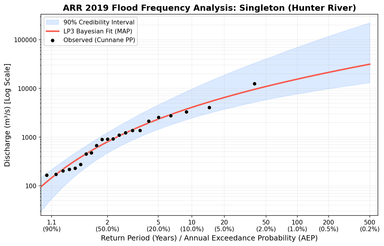
Bayesian Parameter Estimation
Beyond L-moments and LH-moments, pyextremes inherits the upstream library’s MCMC-based Bayesian fitting via emcee. For LP3 this produces full posterior distributions over the three parameters (shape ‘skew’, location μ, scale σ) rather than point estimates — which is directly useful for uncertainty quantification at rare return periods.
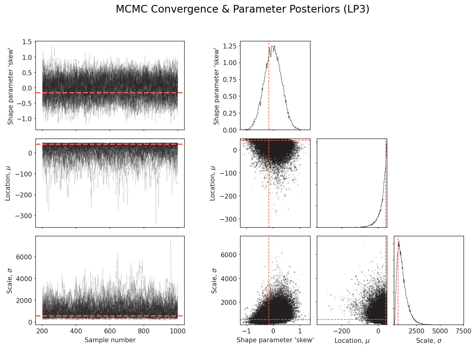
The chain traces (left) show good mixing and stationarity — a necessary condition before reading anything from the posteriors. The joint distributions (right) show the parameter correlation structure: for LP3, location and scale are correlated, while skew is relatively well-constrained. These diagnostics should be checked before accepting any MCMC-derived confidence intervals on the return-period curve.
ARR 2019 Alignment
| pyextremes feature | ARR 2019 reference |
|---|---|
| LP3 via L-moments | Book 3, Chapter 2 — at-site FFA primary distribution |
| Multiple Grubbs-Beck Test | Book 3, Section 2.6 — PILF identification |
| TCEV distribution | Book 3 — mixed-population catchments |
| LH-moments (h=1,2) | Stedinger & Cohn — robust tail estimation |
| GEV alternative fit | Book 3 — alternative distributions |
How to Use It
The branch is installable directly from GitHub:
git clone https://github.com/lmillard79/pyextremes.git
cd pyextremes
git checkout ARR2019_Book3
pip install -e .
The full user guide has a complete end-to-end FFA example. A Jupyter notebook replicating the ARR 2019 Book 3 Section 2.6 worked example is also in the repository.
Feedback Welcome
If you try it on a real gauge record and something doesn’t work — or works differently than expected — please open a GitHub Issue. That’s genuinely useful. The more real-world records it gets tested on, the more robust the PILF detection and LH-moment fitting will become.
Whether the additions eventually make it into the upstream pyextremes library is an open question — ARR 2019 specifics may be too domain-specific for the original maintainer’s scope. But as a standalone fork it’s viable, and the Australian flood hydrology community is the intended audience.
Fork: lmillard79/pyextremes, ARR2019_Book3. Based on Georgy Bocharnikov’s pyextremes (MIT licence).
Related: A Practitioner’s Primer on Bayesian Flood Frequency Analysis · Reading the 2024 Kedron Brook Flood Study