Is Nash-Sutcliffe Efficiency Enough? A Python Comparison of Calibration Metrics for Australian Flood Models

The legacy problem

Nash-Sutcliffe Efficiency (NSE) has been the default goodness-of-fit metric in hydrology since 1970, and it’s still the number most calibration reports lead with. The trouble, documented since at least Chiew and McMahon’s 1993 survey, is that NSE is a sum-of-squared-errors metric dominated by the largest flows in the record. A model can nail the flood peak and still post a poor NSE from noise on the recession limb — or, less obviously, can carry a real systematic bias and still post an excellent NSE, because NSE doesn’t penalise bias and variability the same way it penalises timing.

The fix isn’t to abandon NSE. It’s to stop reporting it alone. Below are four metrics implemented in Python, run against four synthetic hydrographs each engineered with a specific, known deficiency, so you can see exactly which metric catches which problem — and which one doesn’t.

Four metrics and what they each measure

Nash-Sutcliffe Efficiency (Nash & Sutcliffe, 1970):

NSE = 1 - Σ(obs - sim)² / Σ(obs - mean(obs))²

Range (-∞, 1]. Perfect = 1; NSE = 0 means the model is no better than using the observed mean as a constant prediction. Squared-error term means large flows dominate the score — useful for flood peak focus, but it means the metric can’t distinguish why a model is wrong.

Kling-Gupta Efficiency (Gupta et al., 2009; modified by Kling et al., 2012):

KGE = 1 - √[(r-1)² + (β-1)² + (γ-1)²]

where r is the Pearson correlation, β = mean(sim)/mean(obs) is the bias ratio, and γ = CV(sim)/CV(obs) is the ratio of coefficients of variation. KGE’s real value is that it decomposes — when it’s low, you can look at r, β, and γ individually and know immediately whether the problem is timing (r), volume (β), or variability (γ).

Percent Bias (Moriasi et al., 2007):

PBIAS = 100 × Σ(obs - sim) / Σ(obs)

Positive = model underestimates; negative = overestimates. Simple, interpretable, and — as the results below show — blind to timing errors entirely.

Peak flow bias — not a standard named metric, but a useful diagnostic: mean percentage error calculated only at the observed peaks (identified via scipy.signal.find_peaks), rather than across the whole record. For flood engineering, the metric that matters most is often the one restricted to the part of the hydrograph you actually design against.

Python implementation

import numpy as np
from scipy.signal import find_peaks

def nse(obs, sim):
    obs, sim = np.asarray(obs, float), np.asarray(sim, float)
    numerator = np.sum((obs - sim) ** 2)
    denominator = np.sum((obs - obs.mean()) ** 2)
    return np.nan if denominator == 0 else 1.0 - numerator / denominator

def kge(obs, sim):
    obs, sim = np.asarray(obs, float), np.asarray(sim, float)
    r = np.corrcoef(obs, sim)[0, 1]
    beta = sim.mean() / obs.mean()
    gamma = (sim.std() / sim.mean()) / (obs.std() / obs.mean())
    kge_val = 1.0 - np.sqrt((r - 1) ** 2 + (beta - 1) ** 2 + (gamma - 1) ** 2)
    return kge_val, r, beta, gamma

def pbias(obs, sim):
    obs, sim = np.asarray(obs, float), np.asarray(sim, float)
    return 100.0 * np.sum(obs - sim) / np.sum(obs)

def peak_bias(obs, sim, prominence=None):
    obs, sim = np.asarray(obs, float), np.asarray(sim, float)
    if prominence is None:
        prominence = obs.max() * 0.1
    peak_idx, _ = find_peaks(obs, prominence=prominence)
    if len(peak_idx) == 0:
        return np.nan
    return np.mean((sim[peak_idx] - obs[peak_idx]) / obs[peak_idx]) * 100.0

Every function is unit-tested against a known-answer case (perfect model → NSE=KGE=1, PBIAS=0) before being applied to anything real — worth flagging one thing this caught: testing floating-point results for exact equality (kge(...) == 1.0) fails even on a genuinely perfect model, because np.corrcoef on an identical series returns 0.9999999999999999, not 1.0. Use np.isclose() for these tests, not ==.

Applied to four synthetic scenarios

Four single-peaked 72-hour hydrographs, each a variant of the same “observed” event with one specific, known deficiency injected — deliberately chosen to mirror common RORB/URBS calibration failure modes:

A: perfect match. B: simulated volumes 30% too high throughout, correct timing. C: correct shape and volume, peak arrives 6 hours early. D: correct timing, peak flow 40% too low.

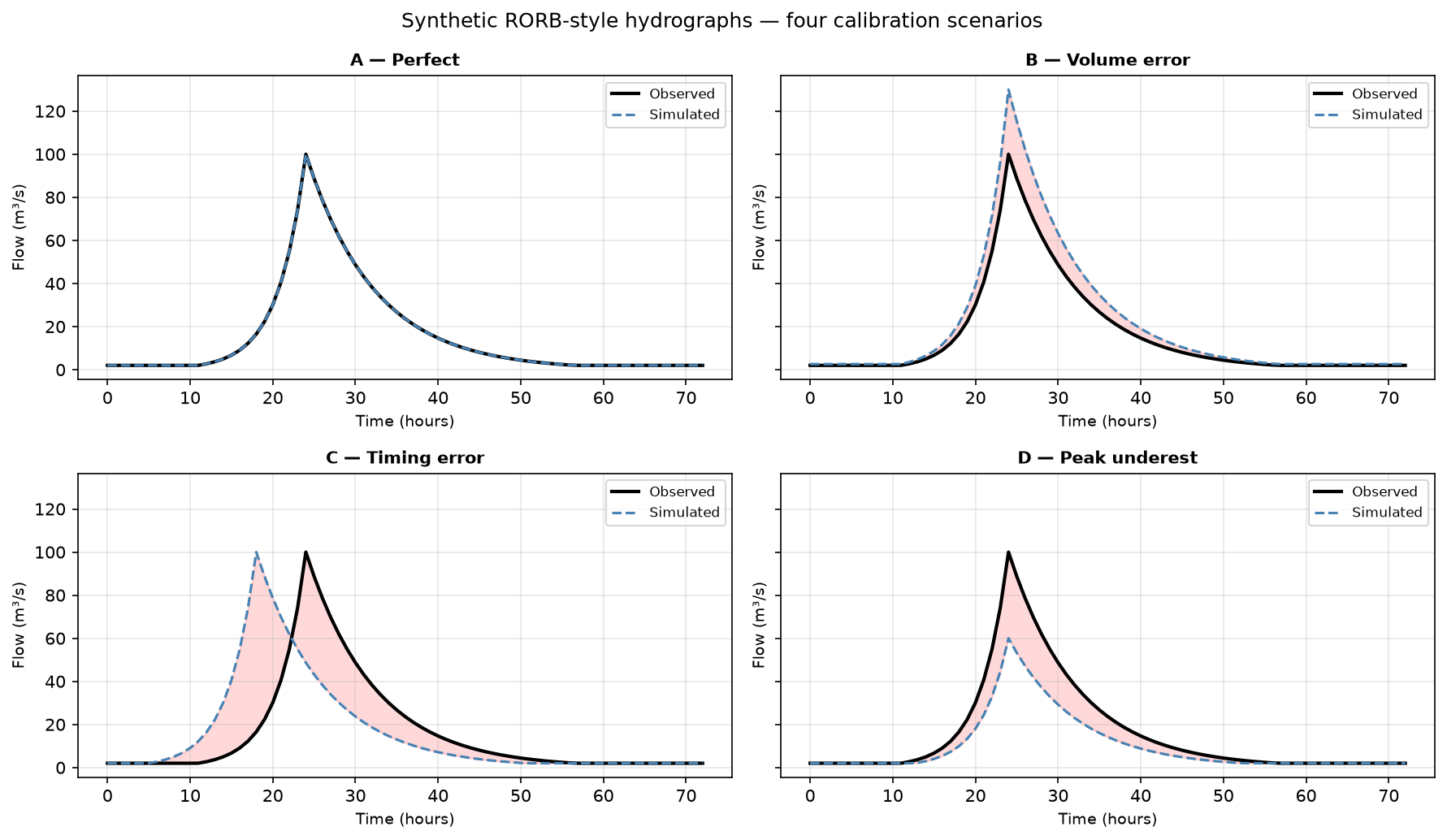
Scored against all four metrics:

Scenario	NSE	KGE	PBIAS (%)	Peak bias (%)
A — Perfect	1.000	1.000	0.0	0.0
B — Volume error (+30%)	0.865	0.700	−30.0	30.0
C — Timing error (−6h)	0.091	0.545	0.0	−51.3
D — Peak underestimate (−40%)	0.760	0.617	38.0	−40.0

Which metric catches which problem?

Each column coloured on its own scale (best-in-column to worst-in-column) — NSE/KGE and PBIAS/peak-bias are different units and aren't comparable on a shared linear scale.

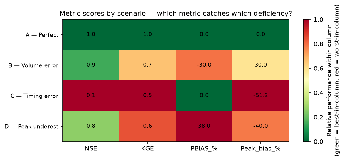
Two results are worth sitting with:

Scenario B (volume error) posts an NSE of 0.865 — “Very Good” by the Moriasi et al. (2015) thresholds used in ARR 2019 calibration reporting — despite a systematic 30% overestimate of every ordinate in the record. NSE’s squared-error formulation is dominated by the timing and shape match, which are perfect here; the consistent volume bias barely dents it. PBIAS catches it instantly (−30%, “Unsatisfactory”). If you report NSE alone, this model passes.

Scenario C (timing error) is the mirror image. PBIAS reports 0.0% — “Very Good” — because a 6-hour shift doesn’t change total volume, only when it arrives. But NSE collapses to 0.091 (“Unsatisfactory”) and peak bias to −51.3%, because at any given timestep the simulated and observed hydrographs are wildly out of phase during the rise. A model with a real, operationally serious timing error would sail through a PBIAS-only check.

KGE’s decomposition (r, β, γ) makes the diagnosis explicit rather than implicit — for scenario C, r = 0.545 immediately points at correlation/timing as the problem, not volume (β = 1.00, correct) or variability (γ = 1.00, correct).

Recommended metric set for ARR 2019 calibration reporting

No single metric here is “wrong” — each is answering a different question, and the pairing matters more than any individual score:

• NSE — overall goodness-of-fit, timing- and shape-sensitive. Report it because it’s the field standard, but never alone.
• PBIAS — catches systematic volume bias that NSE can hide. Cheap to compute, easy to explain to a non-technical reviewer.
• KGE (with its r/β/γ decomposition) — when NSE or PBIAS flags a problem, KGE’s decomposition tells you which of timing, bias, or variability is driving it, without needing a separate diagnostic step.
• Peak flow bias — for flood engineering specifically, the metric computed at the observed peaks only is often more decision-relevant than a whole-of-record statistic, since design outcomes hinge on the peak, not the recession.

Minimum practical set for a calibration report: NSE + PBIAS + KGE decomposition, with peak flow bias added whenever the model’s purpose is flood peak estimation rather than continuous simulation or water balance.

Limitations

• These are synthetic scenarios with one injected deficiency each, chosen for pedagogical clarity — real calibration errors are rarely this clean, and typically combine several of these failure modes at once.
• The Moriasi et al. (2015) thresholds used for classification were developed primarily for continuous water-balance and water-quality models; treat them as a reporting convention, not a pass/fail engineering criterion, particularly for flashy or ephemeral catchments where “satisfactory” NSE is harder to achieve on physical grounds alone.
• Peak flow bias as implemented here depends on the prominence parameter passed to scipy.signal.find_peaks — sensible for a single-event hydrograph, but check it against multi-peak or continuous-simulation records before reusing as-is.

---

Companion notebook: Full implementation, unit tests, and all figures reproducible in notebooks/05_model_performance_metrics/model_performance_metrics.ipynb.

References:

• Gupta, H.V., Kling, H., Yilmaz, K.K. and Martinez, G.F. (2009). Decomposition of the mean squared error and NSE: Implications for improving hydrological modelling. Journal of Hydrology 377(1–2): 80–91.
• Kling, H., Fuchs, M. and Paulin, M. (2012). Runoff conditions in the upper Danube basin under an ensemble of climate change scenarios. Journal of Hydrology 468–469: 264–277.
• Moriasi, D.N. et al. (2007, updated 2015). Model evaluation guidelines for systematic quantification of accuracy in watershed simulations. Transactions of the ASABE 50(3): 885–900.
• Chiew, F.H.S. and McMahon, T.A. (1993). Assessing the adequacy of catchment streamflow yield estimates. Australian Journal of Soil Research 31(5): 665–680.