Sampling ARR 2019 Loss Distributions in Python — A URBS Pre-Processor

The ARR 2019 joint probability framework

ARR 2019 recommends treating initial loss (IL) and continuing loss (CL) as random variables in design flood estimation — sampled via Monte Carlo simulation rather than run once with a fixed median value. The rationale: real catchment losses vary substantially event to event, and a design flood ensemble that treats loss as a constant understates the genuine uncertainty in the resulting flood frequency curve. In practice, most URBS/RORB workflows still use a fixed median IL/CL, because the sampling machinery isn’t built into the model front-ends practitioners actually use day to day. This is a pre-processor to close that gap: draw from ARR’s empirical loss distribution, scale to a catchment’s median, and export in a format ready for a URBS batch run.

The method follows Nathan et al. (2003) and ARR 2019 Book 5, Chapter 3.6.1, and the implementation here is checked against Tony Ladson’s R reference (see The Distribution of Losses).

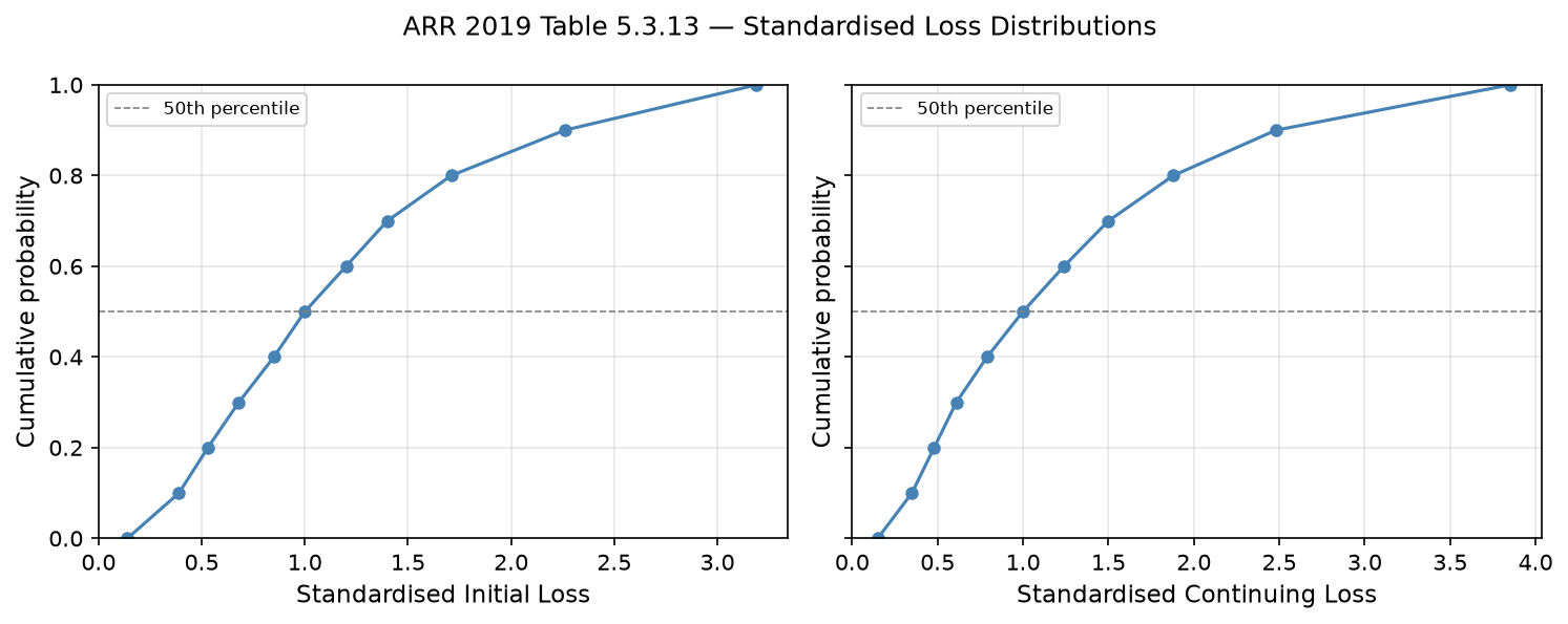
The empirical IL/CL distribution — ARR Table 5.3.13

Table 5.3.13 gives standardised loss values — measured losses divided by each catchment’s own median measured loss — at 11 percentile points, pooled from the dataset behind ARR Project 6 (Hill et al. 2014):

import pandas as pd

loss_std = pd.DataFrame({
    'percentile': [0, 10, 20, 30, 40, 50, 60, 70, 80, 90, 100],
    'prob':       [0, 0.1, 0.2, 0.3, 0.4, 0.5, 0.6, 0.7, 0.8, 0.9, 1.0],
    'IL_std':     [0.14, 0.39, 0.53, 0.68, 0.85, 1.00, 1.20, 1.40, 1.71, 2.26, 3.19],
    'CL_std':     [0.15, 0.35, 0.48, 0.61, 0.79, 1.00, 1.24, 1.50, 1.88, 2.48, 3.85],
})

Standardising this way is what lets one national table serve every catchment: the shape of the distribution is fixed, and you scale it by your catchment’s own median IL/CL (from the ARR Data Hub or your own calibration) to get catchment-specific values.

ARR 2019 Table 5.3.13's standardised loss distributions as empirical CDFs. Both are right-skewed — the tail toward high loss ratios is considerably longer than the tail toward low ones.

Building the sampler: inverse-CDF (quantile function) method

The standard approach — and the one ARR’s own Monte Carlo Simulation Techniques supporting document recommends — is to treat the percentile table as an empirical CDF, build its inverse (the quantile function), and map uniform random draws through it:

from scipy.interpolate import interp1d
import numpy as np

IL_icdf = interp1d(loss_std['prob'], loss_std['IL_std'], kind='linear', bounds_error=True)
CL_icdf = interp1d(loss_std['prob'], loss_std['CL_std'], kind='linear', bounds_error=True)

# Sanity check: the 50th percentile should return 1.0 by construction
print(f"IL at 50th percentile: {IL_icdf(0.5):.3f}  (expected 1.000)")
print(f"CL at 50th percentile: {CL_icdf(0.5):.3f}  (expected 1.000)")

N = 10_000
rng = np.random.default_rng(seed=42)

u_IL = rng.uniform(0, 1, N)
u_CL = rng.uniform(0, 1, N)

IL_samples = IL_icdf(u_IL)
CL_samples = CL_icdf(u_CL)

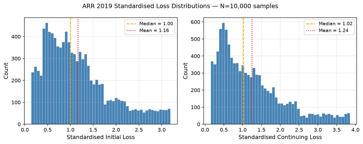
print(f"IL — mean: {IL_samples.mean():.3f}, median: {np.median(IL_samples):.3f}")
print(f"CL — mean: {CL_samples.mean():.3f}, median: {np.median(CL_samples):.3f}")

IL — mean: 1.162, median: 0.997
CL — mean: 1.241, median: 1.018

Ladson’s R implementation reports IL mean ≈1.15/median ≈1.00 and CL mean ≈1.24/median ≈1.00 on the same table — the Python port matches within Monte Carlo sampling noise at N=10,000.

10,000 samples drawn through the inverse CDF. Both distributions show the expected right skew — mean pulled above median by a long tail of high-loss draws.

Scaling to a project’s actual loss values

# Replace with your catchment's actual median IL/CL from the ARR Data Hub
# or your own calibration. Values below are illustrative only.
MEDIAN_IL_mm = 20.0
MEDIAN_CL_mm_hr = 2.5

IL_actual = np.maximum(IL_samples * MEDIAN_IL_mm, 0)      # clip: loss can't be negative
CL_actual = np.maximum(CL_samples * MEDIAN_CL_mm_hr, 0)

print(f"Scaled IL — mean: {IL_actual.mean():.1f} mm, median: {np.median(IL_actual):.1f} mm")
print(f"Scaled CL — mean: {CL_actual.mean():.2f} mm/hr, median: {np.median(CL_actual):.2f} mm/hr")

Scaled IL — mean: 23.2 mm, median: 19.9 mm
Scaled CL — mean: 3.10 mm/hr, median: 2.55 mm/hr

How many ensemble members do you actually need?

Running mean of IL and CL against ensemble size (log scale). Both statistics are still visibly noisy at N=100 (grey dotted line) and don't settle comfortably until several hundred to a thousand members.

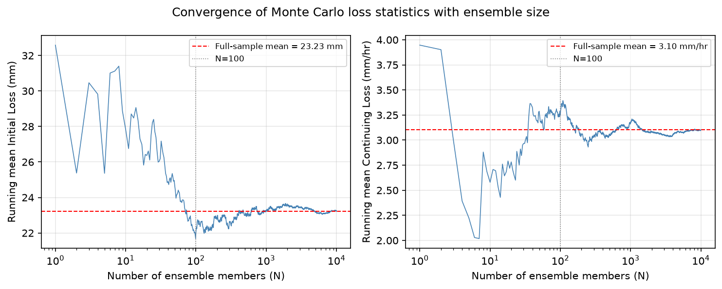
N=100 — a size that’s practical to actually run through URBS/RORB for every ensemble member — is not yet fully converged for either statistic on this table. Worth checking convergence at whatever N your project’s compute budget actually allows, rather than assuming a round number is automatically enough.

Output format for URBS batch input

def export_il_cl_samples(IL_actual, CL_actual, n_members, filepath):
    """Export N IL/CL pairs to CSV for URBS batch input."""
    df = pd.DataFrame({
        'member': np.arange(1, n_members + 1),
        'IL_mm': IL_actual[:n_members].round(1),
        'CL_mm_hr': CL_actual[:n_members].round(2),
    })
    df.to_csv(filepath, index=False)
    return df

for n in [100, 500, 1000]:
    export_il_cl_samples(IL_actual, CL_actual, n_members=n, filepath=f'data/il_cl_samples_N{n:04d}.csv')

Monte Carlo sampling vs. sensitivity testing

These answer different questions, and it’s worth being precise about which one a report is actually presenting. Sensitivity testing — running a handful of discrete loss values, say the 10th/50th/90th percentile — tells you how sensitive the flood estimate is to the loss assumption, holding everything else fixed. Monte Carlo sampling, properly used alongside sampled rainfall depths and temporal patterns in the full ARR joint probability approach, produces an actual flood frequency curve with loss variability propagated through as one of several coupled uncertain inputs. The second is a more defensible basis for a design flood estimate; it’s also more computationally expensive and requires exactly the ensemble machinery above.

Limitations

• Table 5.3.13’s values are national — if your project needs a regionalised loss distribution, this table isn’t automatically the right input; check ARR guidance for your region’s applicability.
• IL and CL are sampled independently here, matching the reference implementation. If your project has evidence of IL/CL correlation for the catchment in question, that’s a real methodological question worth raising with a peer reviewer, not something this pre-processor resolves for you.
• Clipping negative scaled values to zero is a pragmatic fix for the tail of a linear interpolation applied to a bounded physical quantity — reasonable at the volumes here, but worth a sense-check if you’re working with an unusually small median loss where clipping could bite more often.

---

Companion notebook: notebooks/04_monte_carlo_loss_sampling/monte_carlo_loss_sampling.ipynb — includes a section scaffolded for a specific project application (Lower Yarra River RORB calibration), left incomplete pending that project’s own data.

References:

• Ball, J. et al. (2019). Australian Rainfall and Runoff. Book 5, Chapter 3.6.1 and Table 5.3.13.
• Hill, P., Graszkiewicz, Z., Taylor, M., Nathan, R. (2014). Project 6: Loss models for catchment simulation: Phase 4 analysis of rural catchments. ARR Revision Projects.
• Nathan, R.J. et al. (2003). IHWS Proceedings.
• Ladson, A.R. (2019). The Distribution of Losses.