
This post sat as a scaffold for a while. The short-duration Areal Reduction Factor equation was reconstructed, unverified, from a third-party spreadsheet vendor’s published formula; the long-duration equation, its 10 regional coefficient sets, and the interpolation logic for catchments under 10 km² and durations between 12 and 24 hours were all open TODOs, because the ARR 2019 PDF wasn’t directly accessible in the session that started it.
Finding Tony Ladson’s real, working ARR 2019 implementation resolved all of it. As with the rest of this series: the method and the explanation are his (ARR2019 – Areal Reduction Factors and Areal reduction factors – some edge cases); this is a Python port, checked against values he publishes directly, not a reconstruction from a secondary source this time.
What ARFs are for
Point rainfall — an IFD estimate at a single location — systematically overstates the rainfall actually falling, on average, over a large catchment at any given moment, because storm cells don’t cover a whole large catchment with uniform intensity simultaneously. An Areal Reduction Factor (always ≤ 1) corrects for this before a design rainfall depth goes into a URBS, RORB, or WBNM model. Skipping it on anything but a very small catchment systematically overestimates design flood peaks.
The two equations
Short duration (≤12h, one national equation):
import numpy as np

def arf_short(area, duration, aep):
    """ARR 2019 short-duration (<=720 min) Areal Reduction Factor."""
    a, b, c, d = 0.287, 0.265, 0.439, 0.36
    e, f, g = 0.00226, 0.226, 0.125
    h, i, j = 0.0141, -0.021, 0.213
    val = (1
           - a * (area**b - c * np.log10(duration)) * duration**(-d)
           + e * area**f * duration**g * (0.3 + np.log10(aep))
           + h * area**j * 10**(i * (1/1440) * (duration - 180)**2) * (0.3 + np.log10(aep)))
    return min(1.0, val)
This turned out to be identical to what the earlier, unverified draft had reconstructed from a third-party source — every coefficient matches Ladson’s real implementation exactly. Worth knowing, but not something I’d have wanted to publish on the strength of that source alone.
Long duration (24–168h, 10 climatological regions):
REGIONS = {
    'East Coast North':     (0.327,  0.241, 0.448, 0.36,  0.00096,   0.48,   -0.21,  0.012,   -0.0013),
    'Semi-arid Inland QLD': (0.159,  0.283, 0.25,  0.308, 7.3e-07,   1.0,     0.039, 0.0,      0.0),
    'Tasmania':              (0.0605, 0.347, 0.2,  0.283, 0.00076,   0.347,   0.0877,0.012,   -0.00033),
    'SW WA':                 (0.183,  0.259, 0.271,0.33,  3.845e-06, 0.41,    0.55,  0.00817, -0.00045),
    'Central NSW':           (0.265,  0.241, 0.505,0.321, 0.00056,   0.414,  -0.021, 0.015,   -0.00033),
    'SE Coast':               (0.06,   0.361, 0.0, 0.317, 8.11e-05,  0.651,   0.0,   0.0,      0.0),
    'Southern Semi-arid':     (0.254,  0.247, 0.403,0.351, 0.0013,    0.302,   0.058, 0.0,      0.0),
    'Southern Temperate':     (0.158,  0.276, 0.372,0.315, 0.000141,  0.41,    0.15,  0.01,    -0.0027),
    'Northern Coastal':       (0.326,  0.223, 0.442,0.323, 0.0013,    0.58,   -0.374, 0.013,   -0.0015),
    'Inland Arid':            (0.297,  0.234, 0.449,0.344, 0.00142,   0.216,   0.129, 0.0,      0.0),
}

def arf_long(area, duration, aep, region):
    """ARR 2019 long-duration (>=1440 min) Areal Reduction Factor."""
    a, b, c, d, e, f, g, h, i = REGIONS[region]
    val = (1
           - a * (area**b - c * np.log10(duration)) * duration**(-d)
           + e * area**f * duration**g * (0.3 + np.log10(aep))
           + h * 10**(i * area * duration / 1440) * (0.3 + np.log10(aep)))
    return min(1.0, val)
Ten regions, not the 11 an earlier version of this draft’s notes assumed — East Coast North, Semi-arid Inland QLD, Tasmania, SW WA, Central NSW, SE Coast, Southern Semi-arid, Southern Temperate, Northern Coastal, Inland Arid. Climatologically delineated, not by state.
Validated directly against Ladson’s own output
His ARF_edge_cases.R prints two specific values while investigating a real ARR 2019 quirk (below). Both checked here, not eyeballed:
v_short = arf_short(26, 720, 0.0005)
v_long = arf_long(26, 1440, 0.0005, 'Tasmania')
arf_short(26, 720, 0.0005)             = 0.9377527  (Ladson: 0.9377527)
arf_long(26, 1440, 0.0005, 'Tasmania')  = 0.9322746  (Ladson: 0.9322746)
Both match to 7 decimal places.
The part that isn’t obvious from the ARR text
Two things the standard doesn’t spell out clearly, that Ladson’s implementation handles explicitly:
Catchments under 10 km² — neither equation is evaluated directly. Instead, compute the ARF at 10 km² first, then interpolate down to the actual area:
arf_at_10km2 = arf_long(10, duration, aep, region)  # or arf_short, depending on duration
arf_value = 1 - 0.6614 * (1 - arf_at_10km2) * (area**0.4 - 1)
Duration between 12h and 24h — not simply linear interpolation on the ARF value at the target duration. Compute the short-duration ARF at exactly 12h and the long-duration ARF at exactly 24h (both at the target area, or at 10 km² first if area < 10 km²), then interpolate linearly between those two by how far the target duration sits between 720 and 1440 minutes:
arf_short_12 = arf_short(area, 720, aep)
arf_long_24 = arf_long(area, 1440, aep, region)
arf_value = arf_short_12 + (arf_long_24 - arf_short_12) * (duration - 720) / 720
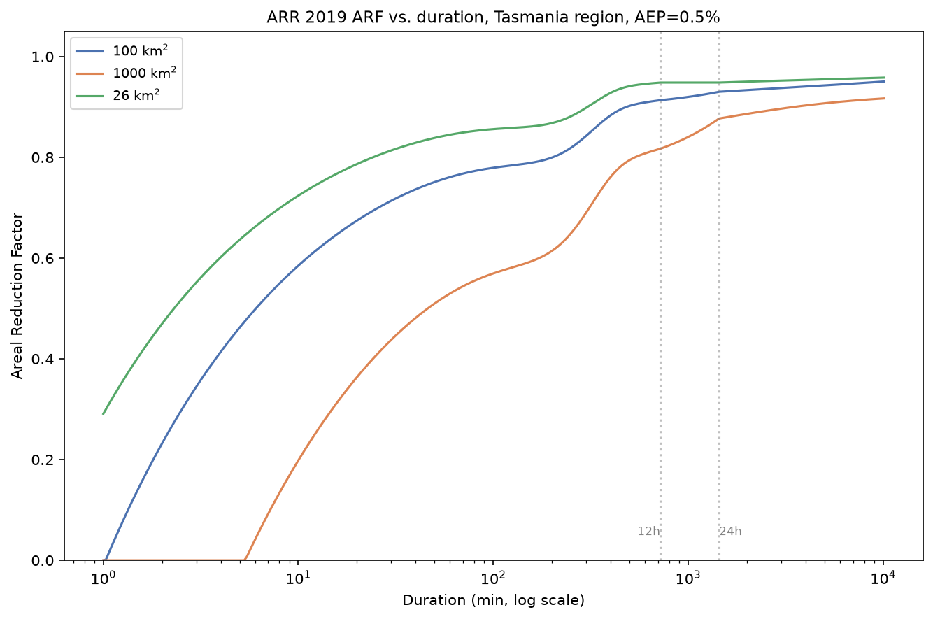
Checking continuity across both boundaries confirms the interpolation is implemented correctly — no visible jump:
Continuity at 12h:  719 min -> 0.8523   720 min -> 0.8523   721 min -> 0.8524
Continuity at 24h:  1439 min -> 0.6254  1440 min -> 0.6256
A genuine ARR 2019 quirk, not a bug
For some catchments, the short-duration ARF at 12h is larger than the long-duration ARF at 24h — the ARF-vs-duration curve briefly slopes downhill right at the transition, rather than monotonically decreasing with duration the way intuition suggests:
26 km² Tasmanian catchment, AEP=0.05%:
  short-duration ARF at 12h = 0.9378
  long-duration ARF at 24h  = 0.9323
  short > long: True
Ladson documents this explicitly in his edge-cases post. It’s a real feature of the two equations meeting at the boundary, not an implementation error — worth knowing before assuming any ARF curve has to be monotonic.
Full validity range
Raises rather than silently extrapolating outside ARR 2019’s stated range: area (0, 30000] km², AEP [0.005, 0.5] (0.5%–50% — not 0.05% as an earlier version of this draft’s notes assumed), duration [0, 10080] min. Short-duration equations are additionally invalid above 1000 km².
Usage: an ARF matrix for a design storm workflow
AREA, REGION = 850, 'East Coast North'
durations_h = [1, 2, 3, 6, 9, 12, 18, 24, 36, 48, 72]
aeps = [0.5, 0.2, 0.1, 0.05, 0.02, 0.01, 0.005]

for dh in durations_h:
    row = [arf(AREA, dh * 60, a, REGION) for a in aeps]
    print(dh, row)
Decreasing ARF at fixed duration as AEP gets rarer (more spatially concentrated storms need more reduction), increasing ARF at fixed AEP as duration lengthens (more spatially uniform) — both directions matching the physical intuition ARFs are meant to capture.
Limitations
- ARF regions are climatological, not administrative — don’t assume a catchment near a region boundary behaves like the interior of either region without checking.
- The equations assume a nominally circular/compact catchment shape typical of ARF derivation methodology; check ARR guidance before applying to strongly elongated catchments without adjustment.
- Valid only within the stated ranges above — the function raises outside them rather than extrapolating.
Companion notebook: notebooks/03_arf_calculator/
Source: Ladson, A.R. (2020). ARR2019 – Areal Reduction Factors; Areal reduction factors – some edge cases. R source: gist.github.com/TonyLadson/fc870cf7ebfe39ea3d1a812bcc53c8fb, gist.github.com/TonyLadson/b8baac6c450fe7f32f5020eb496e8b62.
Reference: Ball, J., Babister, M., Nathan, R., Weeks, W., Weinmann, E., Retallick, M. and Testoni, I. (Editors) (2019). Australian Rainfall and Runoff: A Guide to Flood Estimation. Commonwealth of Australia. Book 2.