
Fifth in an occasional series drawing on Tony Ladson’s blog — his explanation and the underlying method are his; I’m providing a translation for readers who know Python better than R. Usually this series is a fairly direct port of his R, checked against his own published numbers. This one isn’t, and it’s worth being upfront about why.
A note on scope, unlike the rest of this series: the tool I use to fetch his gists declined to reproduce the source for Fitting non-linear models verbatim, citing the original research dataset behind it (an Antecedent Precipitation Index vs. Initial Loss relationship). So what follows is an original Python demonstration of the same general method his post covers, on a different, standard example — a stage-discharge rating curve — with clearly synthetic data, rather than a reconstruction of his dataset from a declined fetch. Read his original post for his actual worked example; this is the Python side of the general technique, not a translation of his specific one.
The problem his post flags
R’s lm() gives you confidence and prediction intervals for free. nls() — the nonlinear equivalent — doesn’t; you need a separate package (he points to propagate::predictNLS) or to propagate the uncertainty yourself. It’s exactly as true in Python: scipy.optimize.curve_fit hands you a point estimate and a covariance matrix, and what you do with the covariance matrix is entirely up to you.
A synthetic rating curve
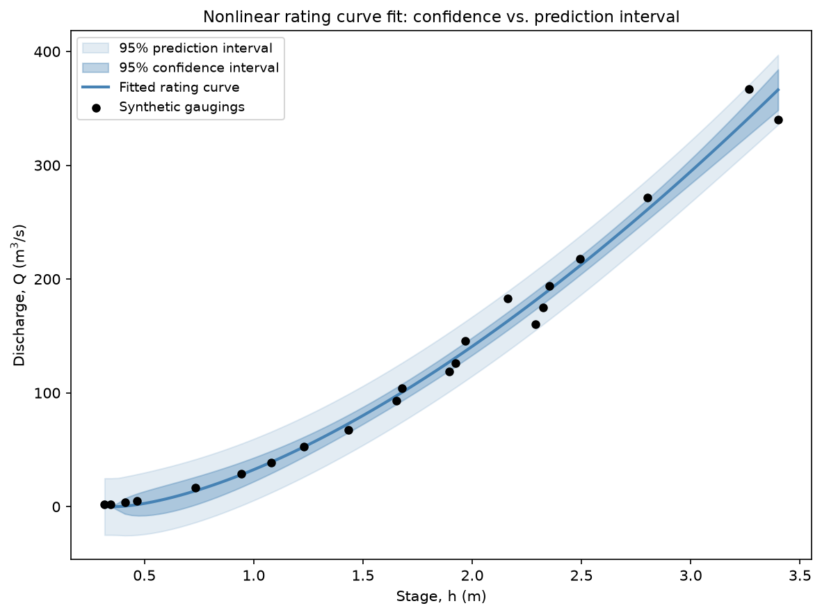
Stage-discharge rating: Q = C·(h − h0)ⁿ — standard power-law form, fit to synthetic gaugings generated from a known “true” relationship plus 6% measurement noise, so there’s a ground truth to check against.
import numpy as np
from scipy import optimize, stats

rng = np.random.default_rng(20260901)
true_C, true_h0, true_n = 45.0, 0.15, 1.85
h_obs = np.sort(rng.uniform(0.3, 3.5, 22))
Q_true = true_C * (h_obs - true_h0) ** true_n
Q_obs = Q_true * (1 + rng.normal(0, 0.06, size=h_obs.size))

def rating_curve(h, C, h0, n):
    return C * np.maximum(h - h0, 1e-6) ** n

popt, pcov = optimize.curve_fit(rating_curve, h_obs, Q_obs, p0=[1.0, 0.0, 2.0], maxfev=10000)
Fitted: C=66.38+/-18.98   h0=0.371+/-0.202   n=1.541+/-0.177
(true:  C=45.0            h0=0.15            n=1.85)
A real gotcha, not the point of the post but worth knowing
The fitted parameters are noticeably off their “true” values — not because the fit failed, but because power-law rating curve parameters are famously correlated with each other:
D = np.sqrt(np.diag(pcov))
corr = pcov / np.outer(D, D)
[[ 1.     0.985 -0.986]
 [ 0.985  1.    -0.950]
 [-0.986 -0.950  1.   ]]
Every pair of parameters is correlated above 0.9 in magnitude. Several different (C, h0, n) combinations trace out nearly the same curve over the range the data actually covers — a well-known feature of this class of model, not a bug in the fit. Which is exactly why it’s worth checking the fitted curve separately from the individual parameters before deciding the fit is good or bad.
Confidence interval vs. prediction interval
- Confidence interval — uncertainty in the fitted curve itself: where the true mean relationship probably sits, given parameter uncertainty.
- Prediction interval — uncertainty in a new individual observation: necessarily wider, since it adds residual scatter on top of parameter uncertainty.
The delta method gets both explicitly: propagate the parameter covariance through the model’s own gradient to get the curve’s variance, then add the residual variance for the prediction interval.
def rating_curve_grad(h, C, h0, n):
    base = np.maximum(h - h0, 1e-6)
    dC = base ** n
    dh0 = -C * n * base ** (n - 1)
    dn = C * base ** n * np.log(base)
    return np.stack([dC, dh0, dn], axis=-1)

resid = Q_obs - rating_curve(h_obs, *popt)
dof = len(h_obs) - len(popt)
resid_var = np.sum(resid**2) / dof

h_grid = np.linspace(h_obs.min(), h_obs.max(), 100)
J = rating_curve_grad(h_grid, *popt)
var_mean = np.einsum('ij,jk,ik->i', J, pcov, J)   # confidence interval variance
se_pred = np.sqrt(var_mean + resid_var)            # prediction interval std error
At h=2.0 m: fitted Q=140.8
  95% CI: (134.9, 150.3)  width=15.4
  95% PI: (116.5, 168.7)  width=52.1
  Confirmed: PI is wider than CI, as it must be.
Companion notebook: notebooks/12_nonlinear_model_fitting/
Topic inspiration: Ladson, A.R. (2016). Fitting non-linear models — this notebook’s specific data and code are original, not a port of his.