
Tony Ladson’s blog has come up as a reference more than once on this site already — his baseflow separation method, his writing on model performance metrics, his work on ARR loss distributions. I learned a lot of practical Australian hydrology from reading his R, and I’d like to start properly returning the favour: porting specific methods from his blog to Python, checked against his own published numbers rather than just “inspired by” them. This is the first one — and the pattern for the whole series: the explanation and the underlying method are his; I’m just providing a hopefully useful translation service for readers who, like me, know Python better than R.
The source is Fitting a probability model to POT data (25 March 2019), with the R source published separately as a gist. Read his original post for the full explanation — what follows is a Python port and my own summary of the method, not a substitute for it.
Why POT needs a different AEP conversion
An annual maximum series gives you exactly one value per year, so a plotting position formula (Cunnane, Weibull, whatever your convention) hands you an empirical AEP directly. A Partial Duration Series — peaks over some threshold, which can produce several events in a wet year and none in a dry one — doesn’t have that property, and a plotting position formula applied naively to it doesn’t give a valid AEP.
The fix Ladson’s post lays out, following ARR 2016/2019 Book 3 Section 2.8.11: work in EY (expected exceedances per year) instead, and only convert to AEP at the end via the Poisson relationship between the two:
# Ladson's R (from the gist)
AEP2EY <- function(AEP) {
  -log(1-AEP)
}
EY2AEP <- function(EY) {
  (exp(EY) - 1)/exp(EY)
}
def aep_to_ey(AEP):
    return -np.log(1 - AEP)

def ey_to_aep(EY):
    return (np.exp(EY) - 1) / np.exp(EY)  # == 1 - exp(-EY)
The exponential fit, via L-moments
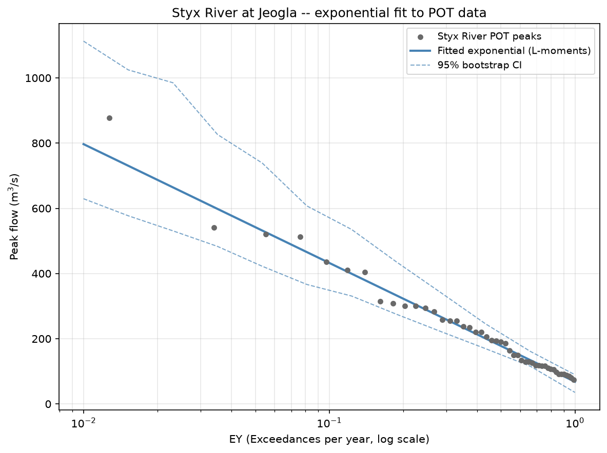
The worked example fits an exponential distribution — parameterised by scale beta and location q_star — using the L-moments method from Wang (1996), on the Styx River at Jeogla partial series (47 peaks). Ladson’s L2() function is the direct sample estimator:
# Ladson's R
L2 <- function(q){
  q <- sort(q)
  n <- length(q)
  0.5*(1/choose(n,2))*sum((0:(n-1) - (n-1):0)*q)
}
from math import comb
import numpy as np

def l2_wang(q):
    """Second L-moment, direct sample estimator (Wang 1996)."""
    q = np.sort(np.asarray(q, dtype=float))
    n = len(q)
    i = np.arange(n)
    weights = i - (n - 1 - i)
    return 0.5 * (1 / comb(n, 2)) * np.sum(weights * q)
Run on the same 47-peak Styx River series he publishes:
styx = np.array([74.0, 79.9, 85.2, 88.6, 91.7, 92.2, 92.2, 98.0, 105.0, 108.0, 111.0,
                  117.0, 117.0, 118.0, 119.0, 126.0, 129.0, 129.0, 134.0, 149.0, 150.0, 164.0,
                  186.0, 190.0, 194.0, 196.0, 206.0, 220.0, 221.0, 235.0, 238.0, 255.0, 255.0,
                  258.0, 283.0, 294.0, 300.0, 301.0, 309.0, 315.0, 405.0, 411.0, 436.0, 513.0, 521.0, 541.0, 878.0])

L1 = styx.mean()
L2 = l2_wang(styx)
beta = 2 * L2
q_star = L1 - beta
L1     = 226.36      (Ladson: 226.36)
L2     = 79.12       (Ladson: 79.12)
beta   = 158.23996   (Ladson: 158.240)
q_star = 68.11748    (Ladson: 68.11748)
Matches to the precision he published.
The flood quantile table
def flood_quantile(EY, beta, q_star, nu=1.0):
    return q_star - beta * np.log(EY / nu)

standard_EY = np.array([1, 0.69, 0.5, 0.22, 0.2, 0.11, 0.05, 0.02, 0.01])
Q = flood_quantile(standard_EY, beta, q_star)
    EY      AEP      ARI        Q     Ladson Q
  1.00   0.6321     1.00     68.1         68.1
  0.69   0.4984     1.45    126.8        127.0
  0.50   0.3935     2.00    177.8        178.0
  0.22   0.1975     4.55    307.7        308.0
  0.20   0.1813     5.00    322.8        323.0
  0.11   0.1042     9.09    417.4        417.0
  0.05   0.0488    20.00    542.2        542.0
  0.02   0.0198    50.00    687.2        687.0
  0.01   0.0100   100.00    796.8        797.0
All nine match his table, including the explicit check value he calls out in a comment: EY=0.01 → 796.8394.
Bootstrap confidence intervals
Ladson uses R’s boot::boot with 5,000 resamples and BCa (bias-corrected and accelerated) intervals. scipy.stats.bootstrap supports the same method directly:
from scipy import stats

def exp_params(q):
    q = np.asarray(q)
    b = 2 * l2_wang(q)
    return b, q.mean() - b

def q01_stat(sample, axis=-1):
    return np.apply_along_axis(lambda s: flood_quantile(0.01, *exp_params(s)), axis, sample)

res = stats.bootstrap((styx,), q01_stat, n_resamples=5000, method='BCa', confidence_level=0.95)
Q at EY=0.01: point=796.84 95% CI=(626, 1109) Ladson: est=796.84, CI=(628, 1132)
Point estimates match exactly, since they’re deterministic. The confidence interval bounds don’t match bit-for-bit — different RNG draws — but land in essentially the same range, which is what you’d want from two independent runs of the same method.
What this checked, and what it didn’t
Every number above that could be checked against Ladson’s own published output was checked, in the notebook itself, with an assertion rather than a visual eyeball — L-moments, fitted parameters, all nine quantiles, the explicit check value, and the bootstrap range. What this port doesn’t independently re-derive is whether the exponential distribution is actually the right model for the Styx River series specifically — that’s a modelling choice inherited from the ARR worked example Ladson’s post follows, not something this notebook re-litigates. The 878 m³/s outlier sitting outside the confidence band is a reasonable prompt to ask that question, not an answer to it.
Companion notebook: notebooks/08_pot_exponential_fit/
Source: Ladson, A.R. (2019). Fitting a probability model to POT data. R source: gist.github.com/TonyLadson/5b01838fef1140293397e23eebe12079.
References:
- Wang, Q.J. (1996). Direct sample estimates of L moments. Water Resources Research 32(12): 3617–3619.
- Ball, J. et al. (2019). Australian Rainfall and Runoff. Book 3, Section 2.8.11.