
After a big flood, “unprecedented” gets used a lot — sometimes accurately, sometimes as a stand-in for “this felt very bad.” Reading the 2024 Kedron Brook Flood Study earlier this year, I found a real, useful counter-example: Brisbane City Council’s consultants worked through exactly this question for the 2022 Brisbane flood events at two Kedron Brook gauges, and found the answer was closer to “rare — roughly 5–10% AEP — not extreme.” That’s a genuinely more useful piece of information than “unprecedented,” and it came from a specific, checkable method: fit the historical record, read off where the new event sits, and run a sensitivity check on how much that one event moves the curve.
This post is the Python mechanics behind that kind of question, generalised: fit a stationary distribution, test the record for trend, and diagnose what a model that assumes nothing has changed would make of a new or recent event.
A data note, upfront: I don’t have access to a real gauge record I can publish here, so everything below runs on synthetic annual-maximum series, disclosed as such throughout. That’s enough to validate that the methods work correctly — it is not a claim about any specific river. Swap in your own project’s annual maximum series and the numbers below become genuinely yours; until then, treat this as the method demonstrated, not a result.
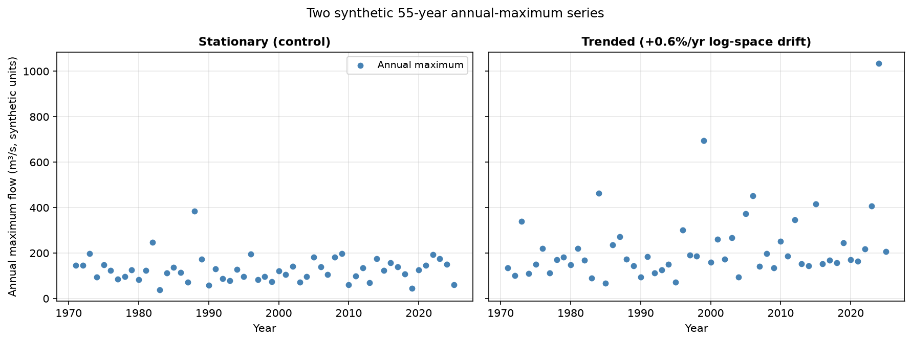
Two synthetic records, one with a trend
Two 55-year annual-maximum series, both drawn from a Log-Pearson III generator — so both are genuinely LP3-distributed by construction, matching what ARR 2019 assumes for Australian at-site flood frequency analysis:
import numpy as np
from scipy import stats

N_YEARS = 55

def make_series(trend_per_year=0.0, seed=0):
    """LP3-distributed annual maxima in log10 space, with optional linear
    drift added to the log-space location term to simulate a trend."""
    rng = np.random.default_rng(seed)
    skew, log_mean, log_sd = 0.3, 2.1, 0.22
    years = np.arange(N_YEARS)
    drift = trend_per_year * years
    log_q = stats.pearson3.rvs(skew=skew, loc=log_mean, scale=log_sd,
                                size=N_YEARS, random_state=rng)
    return 10 ** (log_q + drift)

series_stationary = make_series(trend_per_year=0.0, seed=1)   # control: no trend
series_trended = make_series(trend_per_year=0.006, seed=2)    # 0.6%/yr log-space drift
Fitting the stationary model
scipy.stats.pearson3 parameterises directly as loc/scale/skew — fitting it to log10(annual_max) is Log-Pearson III:
def fit_lp3(annual_max):
    """MLE fit of LP3 (Pearson III on log10-transformed data)."""
    log_q = np.log10(annual_max)
    skew, loc, scale = stats.pearson3.fit(log_q)
    return skew, loc, scale

def lp3_quantile(aep, skew, loc, scale):
    return 10 ** stats.pearson3.ppf(1 - aep, skew=skew, loc=loc, scale=scale)

def lp3_aep(value, skew, loc, scale):
    return 1 - stats.pearson3.cdf(np.log10(value), skew=skew, loc=loc, scale=scale)
ARR 2019 practice often prefers L-moments over MLE for robustness on short records — my pyextremes fork supports that. MLE via plain scipy is enough to demonstrate the diagnostic here without the extra dependency.
Trend testing: Mann-Kendall, and checking the test itself
The Mann-Kendall test is the standard non-parametric trend test in the water-resources literature (Helsel & Hirsch, 2002) — it doesn’t assume a particular distribution, which matters for a right-skewed annual-maximum series. The mechanics: for every pair of observations, count whether the later one is larger, smaller, or tied; sum those signs into a statistic S; compare S to its expected variance under “no trend.” Sen’s slope — the median of all pairwise slopes — gives a trend magnitude that isn’t dragged around by one or two large events the way an ordinary linear regression slope would be.
def mann_kendall(x):
    """Mann-Kendall trend test. Returns S, Z, two-sided p-value, and Sen's slope."""
    n = len(x)
    s = 0
    for k in range(n - 1):
        s += np.sum(np.sign(x[k+1:] - x[k]))
    s = int(s)
    var_s = n * (n - 1) * (2 * n + 5) / 18
    if s > 0:
        z = (s - 1) / np.sqrt(var_s)
    elif s < 0:
        z = (s + 1) / np.sqrt(var_s)
    else:
        z = 0.0
    p = 2 * (1 - stats.norm.cdf(abs(z)))
    slopes = [(x[j] - x[i]) / (j - i) for i in range(n - 1) for j in range(i + 1, n)]
    return s, z, p, float(np.median(slopes))
Before trusting this on anything real, it needs to correctly tell the two synthetic series apart — that’s the actual point of having a known-stationary control:
for name, series in [('Stationary (control)', series_stationary), ('Trended', series_trended)]:
    s, z, p, sen = mann_kendall(series)
    verdict = 'SIGNIFICANT trend (p < 0.05)' if p < 0.05 else 'no significant trend (p >= 0.05)'
    print(f'{name:22s} S={s:5d}  Z={z:+.2f}  p={p:.4f}  Sen\'s slope={sen:+.3f}/yr  -> {verdict}')
Stationary (control)  S=   41  Z=+0.29  p=0.7715  Sen's slope=+0.110/yr  -> no significant trend (p >= 0.05)
Trended                S=  319  Z=+2.31  p=0.0210  Sen's slope=+1.459/yr  -> SIGNIFICANT trend (p < 0.05)
Correctly quiet on the control, correctly flags the trended series at the conventional 5% level. That’s the implementation earning the right to be used on a real record — not a substitute for checking it against a reference implementation before it matters for a real project, but a reasonable first bar.
The percentile diagnostic
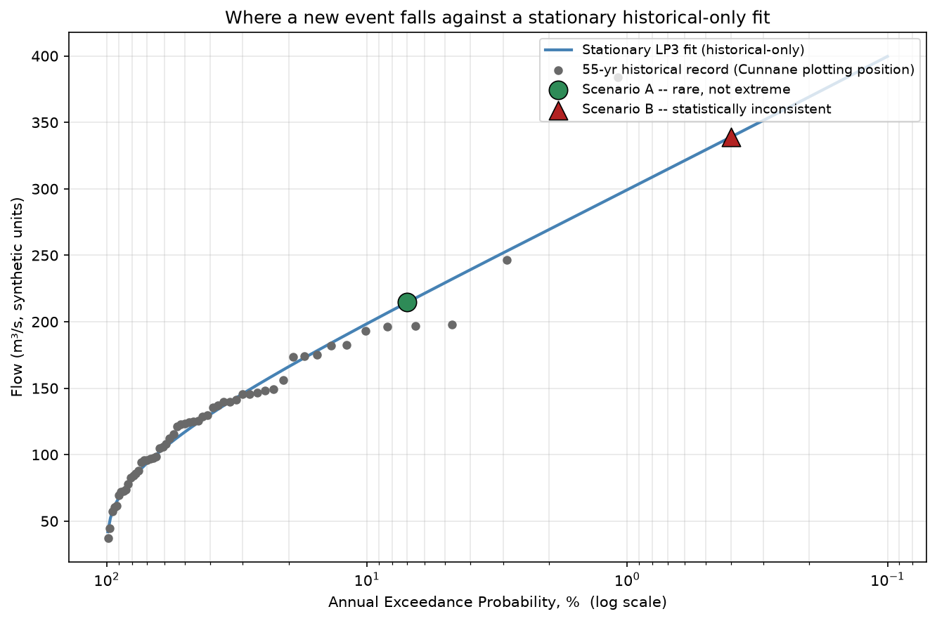
This is the question a “how unusual was that, really” discussion is actually asking, made explicit: fit LP3 to the historical record, then read off what AEP a model that assumes nothing has changed would assign to a given value.
history = series_stationary  # the full 55-yr historical-only record
skew, loc, scale = fit_lp3(history)

target_aeps = {
    'Scenario A -- rare, not extreme': 0.07,
    'Scenario B -- statistically inconsistent': 0.004,
}
for label, target_aep in target_aeps.items():
    value = lp3_quantile(target_aep, skew, loc, scale)
    recovered_aep = lp3_aep(value, skew, loc, scale)
    print(f'{label}: value={value:.1f}, model AEP={recovered_aep*100:.2f}% (~1-in-{1/recovered_aep:.0f} yr)')
Scenario A -- rare, not extreme: value=214.6, model AEP=7.00% (~1-in-14 yr)
Scenario B -- statistically inconsistent: value=338.9, model AEP=0.40% (~1-in-250 yr)
Both values here are constructed, not observed — chosen deliberately to sit at two different points on the curve so the diagnostic has something to show. Scenario A sits in the same AEP territory the real Kedron Brook analysis found for the 2022 Brisbane event: rare, exactly the kind of thing a 55-year record should occasionally produce, nothing in that number alone suggesting the model is wrong. Scenario B sits somewhere a 55-year stationary record essentially never produces — the kind of result that’s a legitimate reason to look closer, the same way the Kedron Brook study’s sensitivity analysis (re-running the FFA with 2022 excluded) was a reason to check how much one event was moving the whole curve.
What this diagnostic can and can’t tell you
What it can do: replace “unprecedented” with an actual, repeatable AEP against a stated model. Flag when a record is being dominated by one or two large values — a legitimate reason to run the same kind of sensitivity check the Kedron Brook study did. Give the trend question a proper non-parametric test rather than an eyeballed slope.
What it can’t do: explain why an event landed where it did. A Scenario-B-type result is consistent with several different explanations — genuine non-stationarity, a short and unrepresentative record, rating-curve error at extreme flows most gauges are never actually calibrated against, or simply an unlucky draw from a correctly-specified stationary distribution (rare events are, by definition, supposed to happen occasionally). Distinguishing between those is a harder and different question than the one this diagnostic answers.
It also isn’t formal climate attribution. Attribution studies — the World Weather Attribution methodology is the best-known example — use climate model ensembles to estimate how much more likely or intense a specific event was made by warming. That’s a materially different question, answered with different tools, by people whose primary discipline is climate science. Running a Mann-Kendall test on an annual maximum series is a legitimate flood-engineering diagnostic; it is not that, and I’d rather say so plainly than let the two blur together.
Limitations
- 55 years is a generous record length by Australian standards. Many real gauge records are shorter, and both the LP3 fit and the trend test should be read with correspondingly wider uncertainty the shorter the record actually is.
- The Mann-Kendall variance formula used here has no tie correction — fine for continuous synthetic data, but real gauge records with rounded or repeated values need the tie-corrected variance term (Helsel & Hirsch, 2002, cover this).
- LP3 fit here uses MLE for simplicity. For a real project, L-moments or LH-moments (see the pyextremes fork post) are generally the more defensible choice on short, possibly outlier-influenced records.
Companion notebook: notebooks/06_ffa_nonstationarity_diagnostic/ — the Mann-Kendall self-validation (control vs. trended series) is asserted in-notebook, not just eyeballed.
Related: Reading the 2024 Kedron Brook Flood Study · Open-Source Flood Frequency Analysis for ARR 2019 — My pyextremes Fork · A Practitioner’s Primer on Bayesian Flood Frequency Analysis · more on the Climate Risk & Non-Stationarity page
References:
- Ball, J. et al. (2019). Australian Rainfall and Runoff. Book 3, Chapter 2.
- Mann, H.B. (1945). Nonparametric tests against trend. Econometrica 13(3): 245–259.
- Kendall, M.G. (1975). Rank Correlation Methods. Griffin.
- Helsel, D.R. & Hirsch, R.M. (2002). Statistical Methods in Water Resources. USGS Techniques of Water-Resources Investigations, Book 4, Chapter A3.
- Brisbane City Council (2024). Kedron Brook Flood Study, Vol. 1 (for information only, not Council policy).